6DOF Spline Fitter

29 november 2025 in

CTech Metrology, Luc Wens

This project was created with Jules.

GITHub : https://github.com/lucwens/SplineFitter

Read the Doc files where Claude/Gemini/ChatGPT made an analysis

Instructions, open command line and

.\.venv\Scripts\activate
pip install -r .\requirements.txt
cd .\Source\
.\main.py

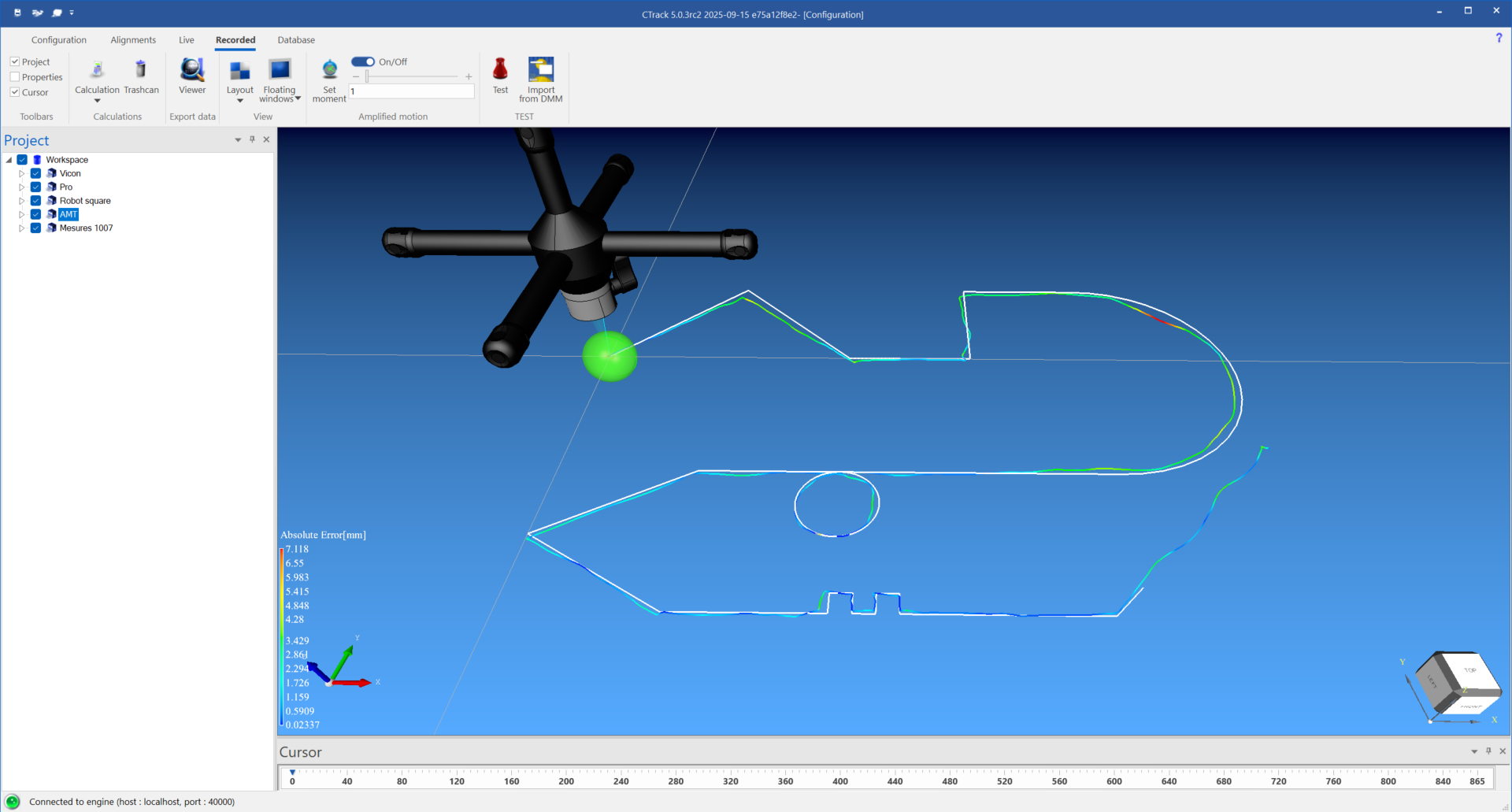
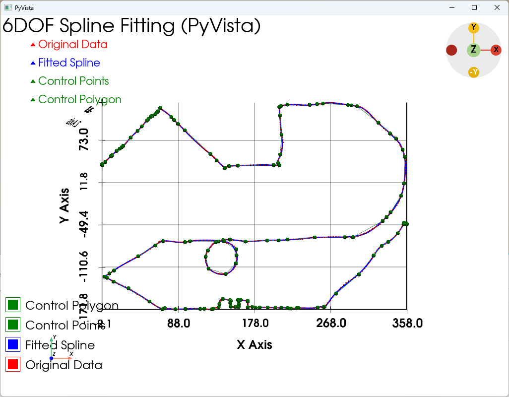
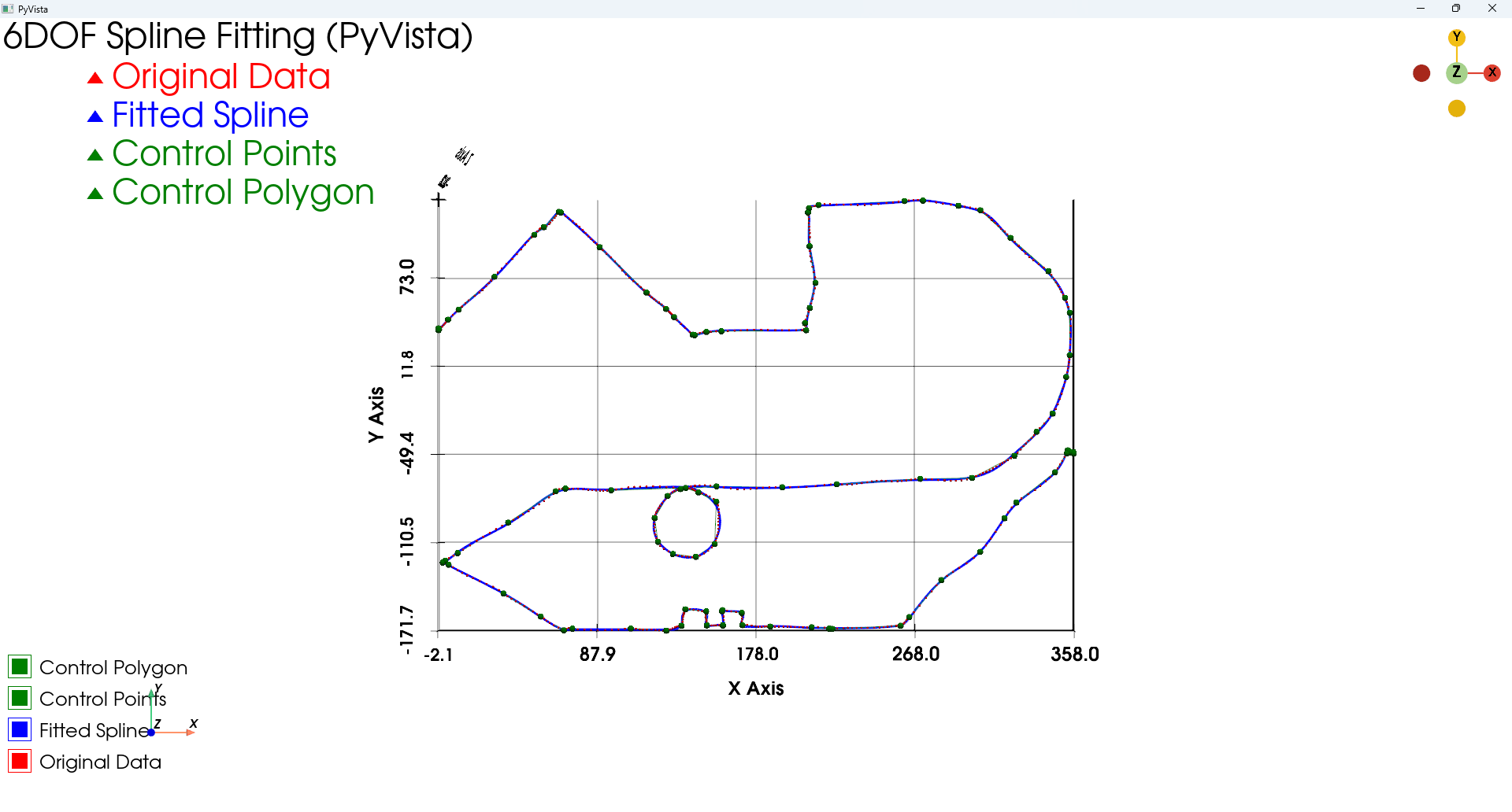
This will create a 3D view with the fitted spline.

I used the data that I captured from a manual run with the MSP over a printed Schmidt path for the AMT conference:

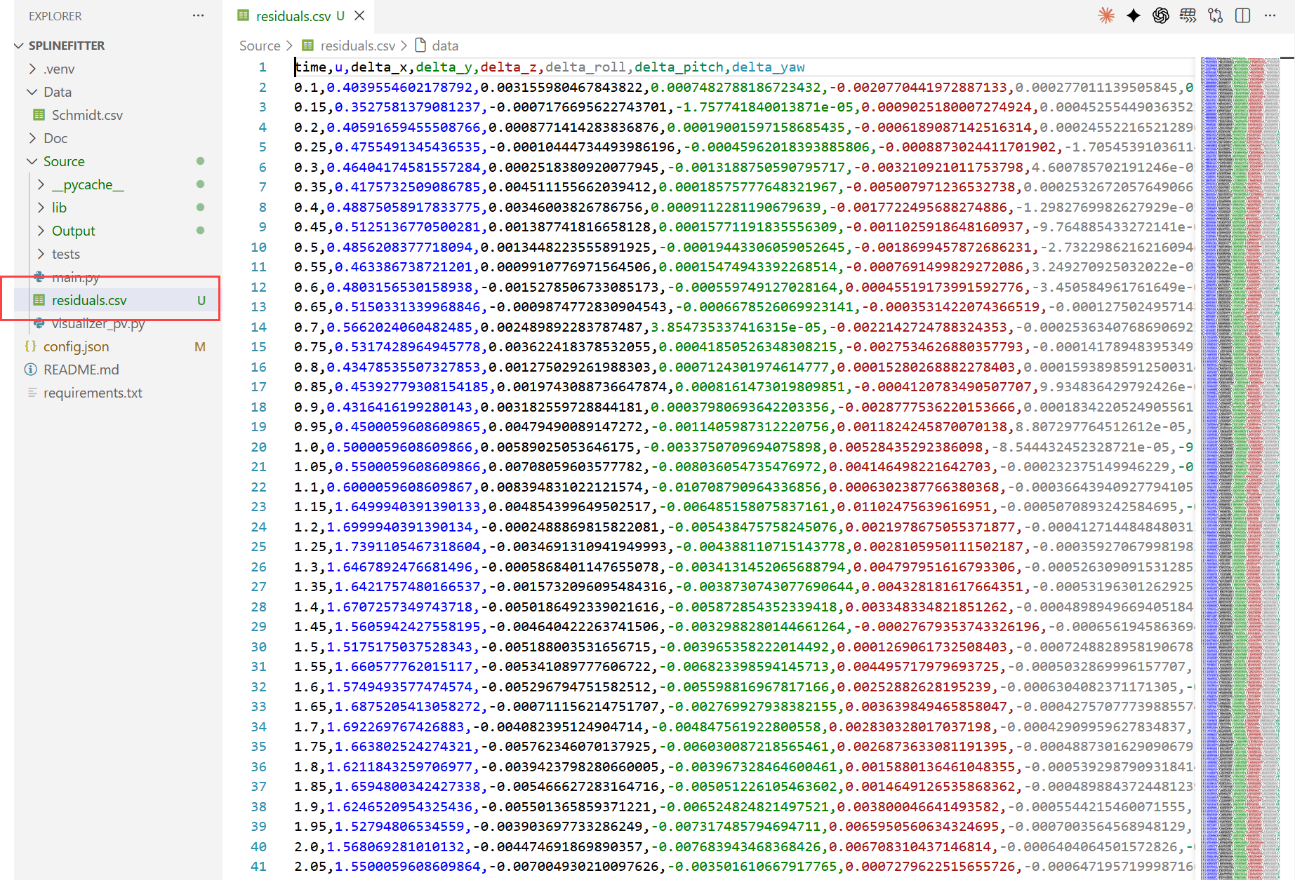
And also an output file with U values and residuals

Use the config.json file to change the behaviour.

{
    "max_gap_duration": 0.5,
    "positional_accuracy": 150.0,
    "rotational_accuracy": 0.5,
    "spline_degree": 3,
    "output_filename": "../residuals.csv"
}

6DOF Spline Fitting Project

This project implements a Python-based pipeline for fitting B-splines to 6-Degree-of-Freedom (6DOF) trajectory data (Position + Orientation). It is designed to handle high-frequency optical tracking data, including potential gaps (NaNs) and varying motion dynamics.

Features

Data Loading & Segmentation: Robustly loads CSV data and segments it based on validity, handling gaps (occlusions) by splitting the trajectory into reliable segments.
Data Reduction: Implements a modified Ramer-Douglas-Peucker (RDP) algorithm for 6DOF data to significantly reduce the number of control points while maintaining trajectory fidelity within specified tolerances.
Spline Fitting:
- Position: Fits cubic B-splines to X, Y, Z coordinates.
- Orientation: Fits splines to orientation data by mapping Unit Quaternions to a Euclidean Tangent Space (using the Logarithmic map), fitting B-splines in that space, and mapping back (Exponential map) to ensure valid rotations.
Visualization: Interactive 3D visualization using PyVista, showing the original noisy data, the smooth fitted spline, and the control points (knots). Supports interactive toggles for visibility.
Analysis: Automatically calculates residuals (deltas) between the measured data and the fitted spline and saves them to a CSV file.
Configuration: All key parameters are configurable via a JSON file.

Directory Structure

Source/
├── data/               # (Optional) Directory for input data
├── lib/                # Core libraries
│   ├── data_loader.py  # Data loading and segmentation logic
│   ├── reduction.py    # 6DOF RDP algorithm
│   ├── spline_fitting.py # Spline fitting logic
│   └── analysis.py     # Residuals calculation
├── tests/              # Unit tests
│   ├── test_loader.py
│   ├── test_reduction.py
│   └── test_spline.py
├── visualizer_pv.py    # PyVista 3D plotting utility
├── main.py             # Main entry point
README.md               # This file
requirements.txt        # Python dependencies
config.json             # Configuration file

Installation

Ensure you have Python 3 installed.
Install the required dependencies:

pip install -r requirements.txt

Configuration

The processing parameters are defined in config.json at the root of the project. You can modify these values to tune the fitting process:

{
    "max_gap_duration": 0.5,       // Maximum duration (seconds) of a gap before splitting segments
    "positional_accuracy": 0.1,    // Tolerance for position error (mm) in RDP reduction
    "rotational_accuracy": 0.5,    // Tolerance for rotational error (degrees) in RDP reduction
    "spline_degree": 3             // Degree of the B-spline (e.g., 3 for cubic)
}

Usage

Running the Main Script

To run the complete pipeline (Load -> Reduce -> Fit -> Visualize):

python3 Source/main.py

The script reads parameters from config.json and expects the data file at Data/Schmidt.csv.

Outputs:

Visualization: An interactive 3D window showing the trajectory.
Residuals: A file Output/residuals.csv containing the calculated errors for every time step:
- time, u: Timestamp (spline parameter).
- delta_x, delta_y, delta_z: Position errors.
- delta_roll, delta_pitch, delta_yaw: Orientation errors (radians).

Running Tests

To verify the correctness of the algorithms:

# From the project root
export PYTHONPATH=$PYTHONPATH:.
python3 Source/tests/test_loader.py
python3 Source/tests/test_reduction.py
python3 Source/tests/test_spline.py

Algorithm Details

1. Data Preprocessing

The DataLoader reads the CSV and checks for NaN values. Continuous sequences of valid data are grouped into Segments. If a gap between valid points exceeds max_gap_duration (default 0.5s), a new segment is created. Small gaps are implicitly bridged during the fitting phase if they are within a segment.

2. Data Reduction (RDP)

The Ramer-Douglas-Peucker (RDP) algorithm is adapted for 6DOF. It recursively splits a trajectory segment if the maximum deviation of intermediate points from the interpolated path (Linear for position, SLERP for rotation) exceeds a threshold.

Position Error: Euclidean distance.
Rotation Error: Geodesic distance (angle) between quaternions.

3. Spline Fitting

Knots: The timestamps of the points retained by the RDP algorithm are used as the knots for the B-spline. This ensures control points are placed where they are most needed (curves, stops).
Orientation Fitting:
1. A reference rotation qrefqref is chosen (first valid point).
2. All orientations qiqi are mapped to a 3D rotation vector ωiωi in the tangent space: ωi=2⋅log⁡(qref−1∗qi)ωi=2⋅log(qref−1∗qi).
3. A cubic B-spline is fitted to the ω(t)ω(t) trajectory.
4. Evaluation converts interpolated ω(t)ω(t) back to quaternions: q(t)=qref∗exp⁡(ω(t)/2)q(t)=qref∗exp(ω(t)/2).

Requirements

numpy
scipy
matplotlib
pandas
pyvista

Some runs

{
    "max_gap_duration": 0.5,
    "positional_accuracy": 20,
    "rotational_accuracy": 20,
    "spline_degree": 3,
    "output_filename": "residuals.csv"
}

{
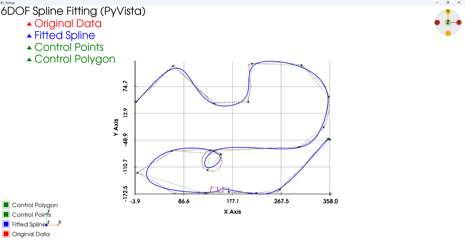
    "max_gap_duration": 0.5,
    "positional_accuracy": 2,
    "rotational_accuracy": 2,
    "spline_degree": 3,
    "output_filename": "residuals.csv"
}

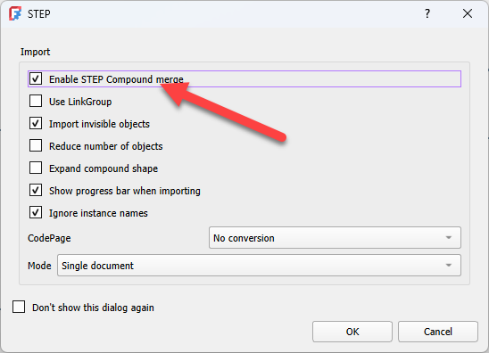
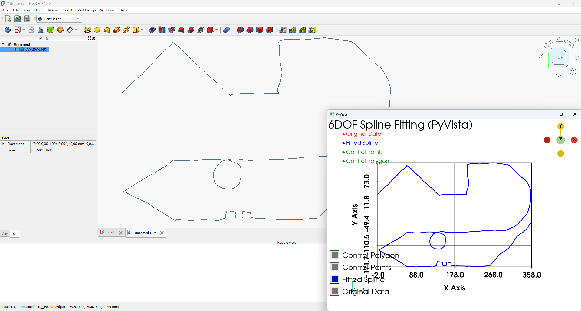
Export to STEP

Make sure to hit the "Compound" option in FreeCAD.

Industrial Robot B-Spline, NURBS & Velocity Control Comparison

Overview

This document provides a comprehensive comparison of how major industrial robot manufacturers handle B-spline curves, NURBS interpolation, and velocity control over complex paths. This is particularly relevant for applications involving:

Playback of recorded 6DOF trajectories
Path teaching from optical tracking/metrology systems
Complex surface following applications
Laser processing, dispensing, and painting

Executive Summary

Key Finding: None of the major industrial robot controllers natively support true B-spline or NURBS interpolation at the controller level. What manufacturers call "spline" motion is typically:

Proprietary smoothing algorithms between taught waypoints
Polynomial corner blending (parabolic or higher-order)
Zone-based trajectory blending

For true B-spline path following with parametric velocity control, external trajectory generation with dense waypoint sampling is required.

Manufacturer Comparison Table

Manufacturer	Controller	Native Spline Type	True B-Spline/NURBS	Velocity Control	Key Commands
KUKA	KRC4/KRC5 (KSS 8.x+)	CP Spline Block (C2-continuous)	❌ No	CONST_VEL, $VEL.CP	SPLINE...ENDSPLINE, SPL, SLIN
FANUC	R-30iB/R-30iB+	CNT/CR blending	❌ No	Per-motion mm/sec, CNT%	L, J, C with CNT/CR/FINE
ABB	IRC5 (RAPID)	Zone-based blending	❌ No	speeddata, zonedata	MoveL, MoveJ, MoveC
Yaskawa	YRC1000 (INFORM)	SplineMove (parabolic)	❌ No	mm/sec per motion	MOVJ, MOVL, MOVC, MOVS
Universal Robots	e-Series (URScript)	MoveP (circular blend)	❌ No	m/s, m/s², blend radius	movej, movel, movec, movep
COMAU	C5G/C5G+ (PDL2)	MOVEFLY blending	❌ No	Per-motion velocity	MOVE, MOVEFLY, MOVE LINEAR
Stäubli	CS8/CS9 (VAL3)	Blend modes	❌ No	mdesc (vel, accel, decel)	movej, movel, movec

Detailed Manufacturer Analysis

KUKA (KRC4/KRC5 - KRL)

Spline Capabilities

KUKA's spline motion is the most advanced among traditional industrial robots, but it is not a true mathematical B-spline. It uses model-based planning to create C2-continuous (smooth up to second derivative) paths through taught waypoints.

Motion Types

krl

; CP Spline Block - Cartesian Path
SPLINE WITH $VEL.CP = 0.5
  SPL point1
  SPL point2 WITH $VEL.CP = 0.3  ; Per-segment velocity
  SLIN point3                     ; Linear segment within spline
  SCIRC aux_point, end_point      ; Circular segment within spline
ENDSPLINE

; PTP Spline Block - Joint Space
PTP_SPLINE
  SPTP point1
  SPTP point2
ENDSPLINE

Velocity Control Features

Feature	Description
$VEL.CP	Cartesian path velocity (m/s)
CONST_VEL	Constant velocity range within spline block
$ACC_AXIS	Joint acceleration limits
$SPL_VEL_RESTR	Cartesian acceleration restriction
TIME_BLOCK	Time-based motion control

Key Characteristics

C2 continuity: Position, velocity, and acceleration are continuous
Model-based planning: Automatically drives as fast as physical limits allow
Path accuracy: No velocity-dependent path deviations
Look-ahead: Full trajectory pre-calculation

Limitations

Teaching positions too close together causes velocity reduction
Mixing legacy (LIN/PTP) and spline motions resets motion planner
Not a true B-spline - internally uses proprietary interpolation

FANUC (R-30iB - TP/KAREL)

Spline Capabilities

FANUC does not have native spline interpolation in the traditional sense. Path smoothing is achieved through:

CNT (Continuous): Percentage-based corner blending (0-100%)
CR (Corner Radius): Geometric radius specification (requires Advanced Motion Package)
S-Motion (v9.30p04+): Paid option for constant velocity through points

Motion Types

fanuc

; Standard motions with blending
L P[1] 500mm/sec CNT100    ; Linear with maximum blending
L P[2] 500mm/sec CR50      ; Linear with 50mm corner radius
J P[3] 100% CNT50          ; Joint with 50% blending
C P[4] P[5] 200mm/sec FINE ; Circular, stop at endpoint

; Arc moves (closest to spline-like behavior)
A P[1] 1000mm/sec CNT100   ; Arc through points

Velocity Control Features

Feature	Description
Speed (mm/sec or %)	Per-motion speed specification
CNT (0-100)	Blending percentage (higher = smoother, less accurate)
CR (mm)	Corner radius (Advanced Motion Package required)
$USEMAXACCEL	Enable fast acceleration feature
S-Motion	Constant velocity through taught points (v9.30+)

Key Characteristics

Trade-off: CNT100 = smooth but path deviation; FINE = accurate but stops
Look-ahead: Requires constants (not variables) for full look-ahead
No true spline: Polynomial corner blending only

Important Notes

CNT value meaning:
- CNT0 = Robot decelerates to stop at point (like FINE)
- CNT100 = Maximum blending, robot may never reach exact point
- CNT is NOT a percentage of velocity

ABB (IRC5 - RAPID)

Spline Capabilities

ABB uses zone-based blending with parabolic corner paths. No native spline interpolation.

Motion Types

rapid

; Motion with zone blending
MoveL p1, v500, z50, tool0;      ! Linear, 50mm zone
MoveJ p2, v1000, z100, tool0;    ! Joint, 100mm zone
MoveC p_via, p3, v200, z10, tool0; ! Circular arc

; Fine positioning (no blending)
MoveL p4, v100, fine, tool0;

; With custom speed
VAR speeddata vCustom := [500, 100, 5000, 1000];
MoveL p5, vCustom, z20, tool0;

Speed Data Structure

rapid

; speeddata = [v_tcp, v_ori, v_leax, v_reax]
; v_tcp: TCP speed in mm/s
; v_ori: Orientation speed in degrees/s
; v_leax: Linear external axis speed in mm/s
; v_reax: Rotating external axis speed in degrees/s

CONST speeddata v500 := [500, 500, 5000, 1000];

Zone Data Structure

rapid

; zonedata controls corner path blending
; Predefined: fine, z0, z1, z5, z10, z15, z20, z30, z40, z50, z60, z80, z100, z150, z200

; fine = stop point (no blending)
; z50 = 50mm zone radius for path blending

Velocity Control Features

Feature	Description
speeddata	TCP velocity, orientation velocity, external axes
zonedata	Corner path blending radius
PathAccLim	Reduce TCP acceleration along path
CorrWrite	Real-time path correction
MultiMove	Synchronized multi-robot velocity

Yaskawa/Motoman (YRC1000 - INFORM)

Spline Capabilities

Yaskawa's SplineMove creates parabolic paths through three taught points. Not a true B-spline.

Motion Types

inform

; Joint interpolation
MOVJ VJ=50.00

; Linear interpolation
MOVL V=500.0

; Circular interpolation
MOVC V=200.0

; Spline interpolation (parabolic through 3 points)
MOVS V=300.0

Velocity Control Features

Feature	Description
V= (mm/sec)	TCP velocity for Cartesian moves
VJ= (%)	Joint velocity percentage
ARATION	Analog output proportional to TCP speed
YMConnect	External streaming interface (YRC1000+)

External Control Options

YMConnect: Buffer-based motion streaming
- Points queued in buffer
- Motion planner interpolates through points
- Same planner as INFORM jobs
- Available on YRC1000 and newer

MotoPlus: Direct controller access
- 4ms interpolation cycle
- mpExRcsIncrementMove for streaming
- Requires WAIT command in INFORM job

Universal Robots (e-Series - URScript)

Spline Capabilities

UR uses MoveP (process move) which provides circular blending between linear segments. Not true spline interpolation.

Motion Types

urscript

# Joint move
movej(target, a=1.4, v=1.05, t=0, r=0)

# Linear move
movel(pose, a=1.2, v=0.25, t=0, r=0)

# Circular move (via point + end point)
movec(pose_via, pose_to, a=1.2, v=0.25, r=0)

# Process move (constant velocity, circular blending)
movep(pose, a=1.2, v=0.25, r=0.05)

Parameters

Parameter	Description
a	Acceleration (m/s² for Cartesian, rad/s² for joint)
v	Velocity (m/s for Cartesian, rad/s for joint)
t	Time (seconds) - overrides a and v if specified
r	Blend radius (meters)

Real-Time Control

urscript

# Servo control at 500Hz
servoj(q, a, v, t=0.008, lookahead_time=0.1, gain=300)

# Path offset overlay
path_offset_set(offset, type)
path_offset_set_alpha_filter(alpha)  # Smooth offset velocity

Key Characteristics

500Hz control loop (e-Series)
MoveP: Accelerates to constant velocity, circular blends
servoj: Real-time streaming at 125Hz or 500Hz
path_offset_*: Real-time path modification overlay

COMAU (C5G/C5G+ - PDL2)

Spline Capabilities

COMAU uses MOVEFLY for fly-by point blending. The Open Controller (C5GOpen) allows external trajectory generation including NURBS.

Motion Types

pdl2

; Standard moves
MOVE TO position
MOVE LINEAR TO position
MOVEFLY TO position  ; Fly-by (blending)

; With speed control
$ARM_SPD_OVR := 50  ; 50% speed override
MOVE LINEAR TO position WITH $MOVE_SPD = 500

Open Controller (C5GOpen)

ORL Motion (ORLM): External trajectory library
- Simulates CRC motion algorithms
- Allows NURBS trajectory generation externally
- Requires specific license
- Real-time communication at 400µs cycle

Stäubli (CS8/CS9 - VAL3)

Spline Capabilities

Stäubli uses motion descriptors (mdesc) with blend modes for path smoothing. No native spline.

Motion Types

val3

// Motion descriptor defines motion parameters
mdesc mNomSpeed
mNomSpeed.vel = 100        // Velocity (% or mm/s)
mNomSpeed.accel = 100      // Acceleration
mNomSpeed.decel = 100      // Deceleration
mNomSpeed.blend = joint    // Blend mode: joint/Cartesian/off
mNomSpeed.leave = 50       // Leave distance (mm)
mNomSpeed.reach = 50       // Reach distance (mm)

// Motions
movej(jTarget, tTool, mNomSpeed)
movel(pTarget, tTool, mNomSpeed)
movec(pVia, pTarget, tTool, mNomSpeed)

Blend Modes

Mode	Description
joint	TCP trajectory unconstrained between leave/reach
Cartesian	TCP stays on plane between leave/reach
off	No blending (stop at point)

NURBS Support in Industrial Robotics

Current State

No major industrial robot controller natively supports NURBS interpolation. Research implementations exist but require:

External NURBS interpolation - Calculate points on the curve externally
Dense waypoint streaming - Feed sampled points to robot controller
Real-time interfaces - Use streaming protocols for high-fidelity reproduction

Research Approaches

Academic and industrial research has demonstrated NURBS interpolation on robots using:

Approach	Description	Complexity
Waypoint sampling	Sample NURBS at intervals, send as waypoints	Low
Real-time streaming	Stream interpolated positions at controller cycle rate	High
Custom controller	Implement NURBS kernel on open controller	Very High

Typical NURBS Implementation Flow

1. Define NURBS curve with control points and knot vector
2. Determine chord error tolerance
3. Adaptively sample curve to meet tolerance
4. Calculate velocity from parametric spacing
5. Generate manufacturer-specific motion commands
6. Upload/stream to robot controller

Velocity Profile Control Strategies

For 6DOF B-Spline with U-Parameterized Velocity

Given a B-spline with:

Control points in 6DOF (position + orientation)
u.txt mapping measurement points to spline parameter u
Implicit velocity profile from u-spacing

Strategy 1: Dense Waypoint Sampling

For each u value in u.txt:
    1. Evaluate B-spline at u → 6DOF pose
    2. Calculate velocity from Δu and original timestamps
    3. Output as motion command with velocity

Pros: Works on all robots, preserves timing Cons: May hit point limits, dense paths slow controllers

Strategy 2: Per-Segment Velocity (KUKA/ABB)

python

# Calculate inter-segment velocities
for i in range(len(u_values) - 1):
    dt = timestamps[i+1] - timestamps[i]
    ds = arc_length(spline, u_values[i], u_values[i+1])
    velocity[i] = ds / dt

Pros: Native controller interpolation Cons: Not all manufacturers support per-segment velocity

Strategy 3: External Streaming

Robot	Interface	Cycle Rate
KUKA	RSI (Robot Sensor Interface)	4ms
FANUC	J519 (Stream Motion)	8ms
ABB	EGM (Externally Guided Motion)	4ms
Yaskawa	YMConnect / MotoPlus	4ms
UR	RTDE	2ms (500Hz)

Pros: Highest fidelity path reproduction Cons: Requires real-time system, most complex

Strategy 4: Time-Based Motion

krl

; KUKA TIME_BLOCK example
SPLINE WITH TIME_BLOCK
  SPL point1
  SPL point2 WITH $SPL_TIME = 0.5  ; 0.5 seconds for this segment
ENDSPLINE

Pros: Direct timing control Cons: Limited manufacturer support

Post-Processor Architecture Recommendations

Generic Post-Processor Structure

cpp

class RobotPostProcessor {
public:
    struct Waypoint6DOF {
        double x, y, z;           // Position (mm)
        double rx, ry, rz;        // Orientation (degrees or radians)
        double velocity;          // Calculated from u-spacing
        double blend_radius;      // Zone/CNT parameter
    };
    
    virtual std::string generateProgram(
        const BSpline6DOF& spline,
        const std::vector<double>& u_values,
        const std::vector<double>& timestamps
    ) = 0;
    
protected:
    std::vector<Waypoint6DOF> sampleSpline(
        const BSpline6DOF& spline,
        const std::vector<double>& u_values,
        const std::vector<double>& timestamps
    ) {
        std::vector<Waypoint6DOF> waypoints;
        
        for (size_t i = 0; i < u_values.size(); ++i) {
            auto pose = spline.evaluate(u_values[i]);
            
            Waypoint6DOF wp;
            wp.x = pose.position.x;
            wp.y = pose.position.y;
            wp.z = pose.position.z;
            wp.rx = pose.orientation.rx;
            wp.ry = pose.orientation.ry;
            wp.rz = pose.orientation.rz;
            
            // Calculate velocity from timing
            if (i > 0) {
                double dt = timestamps[i] - timestamps[i-1];
                double ds = distance(waypoints.back(), pose);
                wp.velocity = ds / dt;
            }
            
            waypoints.push_back(wp);
        }
        return waypoints;
    }
};

KUKA Post-Processor Example

cpp

class KukaPostProcessor : public RobotPostProcessor {
public:
    std::string generateProgram(
        const BSpline6DOF& spline,
        const std::vector<double>& u_values,
        const std::vector<double>& timestamps
    ) override {
        auto waypoints = sampleSpline(spline, u_values, timestamps);
        
        std::stringstream ss;
        ss << "DEF SplineProgram()\n";
        ss << "$TOOL = TOOL_DATA[1]\n";
        ss << "$BASE = BASE_DATA[1]\n\n";
        
        ss << "SPLINE\n";
        for (size_t i = 0; i < waypoints.size(); ++i) {
            const auto& wp = waypoints[i];
            ss << "  SPL {X " << wp.x 
               << ", Y " << wp.y 
               << ", Z " << wp.z
               << ", A " << wp.rx 
               << ", B " << wp.ry 
               << ", C " << wp.rz << "}";
            
            if (wp.velocity > 0) {
                ss << " WITH $VEL.CP = " << wp.velocity / 1000.0;  // m/s
            }
            ss << "\n";
        }
        ss << "ENDSPLINE\n";
        ss << "END\n";
        
        return ss.str();
    }
};

ABB Post-Processor Example

cpp

class AbbPostProcessor : public RobotPostProcessor {
public:
    std::string generateProgram(
        const BSpline6DOF& spline,
        const std::vector<double>& u_values,
        const std::vector<double>& timestamps
    ) override {
        auto waypoints = sampleSpline(spline, u_values, timestamps);
        
        std::stringstream ss;
        ss << "MODULE SplineModule\n";
        ss << "  PROC main()\n";
        ss << "    ConfL \\Off;\n";
        ss << "    SingArea \\Wrist;\n\n";
        
        for (size_t i = 0; i < waypoints.size(); ++i) {
            const auto& wp = waypoints[i];
            
            // Create robtarget
            ss << "    CONST robtarget p" << i << " := [["
               << wp.x << "," << wp.y << "," << wp.z << "],"
               << "[" << quaternionFromEuler(wp.rx, wp.ry, wp.rz) << "],"
               << "[0,0,0,0],[9E9,9E9,9E9,9E9,9E9,9E9]];\n";
            
            // Create speeddata
            ss << "    CONST speeddata v" << i << " := ["
               << wp.velocity << ",500,5000,1000];\n";
            
            // Motion command
            std::string zone = (i == waypoints.size() - 1) ? "fine" : "z10";
            ss << "    MoveL p" << i << ", v" << i << ", " << zone << ", tool0;\n\n";
        }
        
        ss << "  ENDPROC\n";
        ss << "ENDMODULE\n";
        
        return ss.str();
    }
};

Orientation Interpolation Considerations

Challenge

Robot controllers typically use linear interpolation (SLERP-like) between orientation waypoints. Your B-spline may use different orientation interpolation, leading to:

Path deviation in orientation
Need for denser sampling in high-curvature orientation regions

Solutions

Denser sampling: Increase sampling density where orientation changes rapidly
Quaternion representation: Use quaternions for smoother interpolation
Orientation velocity limits: Some controllers limit orientation change rate

cpp

// Check orientation change rate
double orientationChangeRate(const Waypoint6DOF& a, const Waypoint6DOF& b, double dt) {
    // Calculate angular velocity
    Quaternion qa = eulerToQuaternion(a.rx, a.ry, a.rz);
    Quaternion qb = eulerToQuaternion(b.rx, b.ry, b.rz);
    double angle = qa.angularDistanceTo(qb);
    return angle / dt;  // rad/s
}

// Adaptive resampling for orientation
std::vector<double> adaptiveResample(
    const BSpline6DOF& spline,
    const std::vector<double>& u_values,
    double maxOrientationRate  // rad/s
) {
    std::vector<double> newUValues;
    // Add intermediate u values where orientation changes too fast
    // ...
}

Controller Cycle Time Reference

Manufacturer	Controller	Typical Cycle Time	Notes
KUKA	KRC4/KRC5	4-12 ms	RSI at 4ms
FANUC	R-30iB	8 ms	Stream Motion at 8ms
ABB	IRC5	4 ms	EGM at 4ms
Yaskawa	YRC1000	4 ms	MotoPlus default
Universal Robots	e-Series	2 ms	RTDE at 500Hz
COMAU	C5G+	0.4 ms	Open controller
Stäubli	CS9	4 ms	-

Important: If your u-samples are denser than the controller cycle time, you may need to:

Downsample the trajectory
Use the robot's built-in interpolation
Stream points in real-time

Glossary

Term	Definition
B-spline	Basis spline - parametric curve defined by control points and basis functions
NURBS	Non-Uniform Rational B-Spline - generalization of B-splines with weighted control points
CNT	Continuous (FANUC) - percentage-based corner blending
Zone	ABB's term for corner blending region
Blend Radius	Distance from waypoint where blending begins/ends
CP	Continuous Path - motion mode maintaining constant TCP velocity
PTP	Point-to-Point - joint-interpolated motion
RSI	Robot Sensor Interface (KUKA) - real-time external control
EGM	Externally Guided Motion (ABB) - real-time path correction
RTDE	Real-Time Data Exchange (UR) - real-time communication interface

References

KUKA System Software 8.x Operating and Programming Instructions
FANUC Robot Series Operator's Manual
ABB RAPID Reference Manual
Yaskawa INFORM Language Manual
Universal Robots URScript Manual
COMAU PDL2 Programming Language Manual
Stäubli VAL3 Reference Manual

Document created: November 2025 For applications involving optical tracker trajectory playback and 6DOF B-spline path reproduction

Intellectual Property Protection Strategy

Nominal Path Correction Algorithm for Robot Trajectory Compensation

This document outlines strategies for protecting the intellectual property (IP) related to the nominal path correction algorithm developed for robot trajectory compensation.

A self-registred mail was sent on 1/12/2025 with the letter and the source code.

This can be found on

d:\dropbox\ctech\patents\spline fitting
https://github.com/lucwens/SplineFitter/tree/main/Doc

Overview of Protection Options
Immediate Actions - Evidence of Invention
Belgian Patent Protection
European Patent Protection
International Patent Protection
Trade Secret Protection
Recommended Timeline
Sample Registered Letter Text
Comparison Table
Fiscal Advantages - Belgian Innovation Income Deduction

Overview of Protection Options

Types of IP Protection Available

Type	What it Protects	Duration	Cost Range
Patent	Technical invention/method	20 years	€5,000 - €50,000+
Trade Secret	Confidential know-how	Unlimited (if kept secret)	Low (internal costs)
Copyright	Code implementation	70 years after author's death	Free (automatic)
Prior Art Evidence	Establishes invention date	N/A	€10 - €100

What Can Be Protected?

For this algorithm, potentially patentable elements include:

The method of calculating trajectory corrections by applying inverse error vectors
The combination of 6DOF spline fitting with error compensation
The specific implementation of orientation correction in tangent space
The iterative refinement process for high-precision applications

Immediate Actions - Evidence of Invention

Option 1: Registered Letter to Yourself (i-DEPOT Alternative)

Cost: €5-10 (postage)

Timeline: Immediate

Legal Standing: Limited but useful as supporting evidence

Send a sealed, registered letter to yourself containing:

Technical description of the invention
Date of conception
Inventor name(s)
Supporting documentation (code, diagrams)

Important: Do NOT open the letter. The sealed postal date stamp serves as evidence.

Option 2: i-DEPOT (Benelux Office for Intellectual Property)

Cost: €37 (online) or €47 (paper) for 5 years

Timeline: Same day (online)

Legal Standing: Official evidence of existence at a specific date

Website: https://www.boip.int/en/entrepreneurs/ideas/i-depot

Advantages:

Officially recognized in Benelux
Can be renewed indefinitely
Digital storage option
Accepted by courts as evidence

Option 3: Notarized Document

Cost: €50-150

Timeline: Same day

Legal Standing: Strong legal evidence

Have a notary certify the existence and content of your technical documentation on a specific date.

Belgian Patent Protection

Belgian National Patent

Filing Office: Belgian Office for Intellectual Property (OPRI/BOIP)

Website: https://economie.fgov.be/en/themes/intellectual-property/patents

Costs (Approximate)

Stage	Official Fees	Attorney Fees (Optional)
Filing	€50	€2,000 - €4,000
Search Report	€300	Included above
Annual Fees (Years 3-20)	€40 - €600/year	-
Total (20 years)	~€3,000	€5,000 - €8,000

Process

File application with OPRI (description, claims, abstract, drawings)
Formal examination (2-3 months)
Search report issued (novelty assessment)
Publication at 18 months from filing
Grant (no substantive examination in Belgium)

Limitations

No substantive examination: Belgian patents are granted without verifying novelty/inventiveness
Limited territorial scope: Only valid in Belgium
Weak enforcement: Courts may invalidate during litigation

European Patent Protection

European Patent (EP) via European Patent Office (EPO)

Filing Office: European Patent Office

Website: https://www.epo.org

Costs (Approximate)

Stage	Official Fees	Attorney Fees
Filing + Search	€1,400	€3,000 - €6,000
Examination	€1,880	€2,000 - €4,000
Grant + Validation	€900 + validation costs	€1,000 - €2,000
Validation (per country)	€200 - €1,500/country	€300 - €800/country
Annual fees	Varies by country	-
Total (8 key countries, 10 years)	~€25,000 - €35,000	€8,000 - €15,000

Process Timeline

Filing (Month 0)
Search Report (Month 6-9)
Publication (Month 18)
Examination Request (within 6 months of search report)
Examination (2-4 years from filing)
Grant (Month 36-60)
Validation in chosen countries (within 3 months of grant)

Key Countries for Validation

Consider validating in countries with:

Major manufacturing (Germany, France, Italy)
Key competitors' locations
Important markets for robotics

Unitary Patent (UP) - New Option (June 2023)

Coverage: 17 EU member states with single validation

Cost Advantage: Single annual fee instead of per-country fees

Stage	Fees
UP Registration	€0 (no additional filing fee)
Annual Fees (single fee)	€5,000 total over 20 years

Note: Does not cover Spain, Poland, or non-EU countries (UK, Switzerland, etc.)

International Patent Protection

PCT (Patent Cooperation Treaty) Application

Administered by: World Intellectual Property Organization (WIPO)

Website: https://www.wipo.int/pct/en/

The PCT provides a unified filing procedure for 157 countries, delaying national phase costs by 30-31 months.

Costs

Stage	Official Fees	Attorney Fees
International Filing	€1,500 - €2,000	€3,000 - €5,000
International Search	€2,000 - €2,500	Included above
International Publication	Included	-
National Phase (per region)	Varies	€2,000 - €5,000/region

Timeline

Filing (Month 0) - Priority date established
International Search Report (Month 3-4)
International Publication (Month 18)
National/Regional Phase Entry (Month 30-31)
National Examination in each country (Years 2-5)

Major Economic Areas - National Phase Costs

Region/Country	Official Fees	Attorney Fees	Annual Fees (20 yrs)
USA	2,000−2,000−3,000	5,000−5,000−15,000	$15,000
Europe (EP)	€3,000 - €5,000	€8,000 - €15,000	€20,000+
China	500−500−1,000	2,000−2,000−5,000	$3,000
Japan	1,500−1,500−2,500	4,000−4,000−8,000	$10,000
South Korea	500−500−1,000	2,000−2,000−4,000	$5,000

Trade Secret Protection

When to Consider Trade Secrets

Trade secret protection may be preferable if:

The innovation is difficult to reverse-engineer
You can maintain strict confidentiality
The technology evolves rapidly (patents may become obsolete)
Patent enforcement would be difficult

Implementation Steps

Identify confidential information
Mark documents as "CONFIDENTIAL" or "TRADE SECRET"
Restrict access on a need-to-know basis
Use NDAs with employees, contractors, and partners
Implement technical security measures
Document your trade secret protection efforts

Sample NDA Clause for Algorithm

"Confidential Information" includes, but is not limited to, the nominal path
correction algorithm, including the method of calculating trajectory corrections
by applying inverse error vectors to 6DOF spline representations, the specific
implementation of orientation correction in tangent space, and all related
technical documentation, source code, and know-how.

Recommended Timeline

Phase 1: Immediate (Week 1)

Send registered letter to yourself with technical description
File i-DEPOT online (€37)
Conduct preliminary patent search (espacenet.com, Google Patents)

Phase 2: Short-term (Month 1-3)

Consult patent attorney for patentability assessment
Decide on filing strategy
Prepare draft patent application

Phase 3: Filing (Month 3-12)

File Belgian national patent OR
File European patent application OR
File PCT application (if international protection needed)

Phase 4: International (Month 12-30)

Respond to search report
Decide on national phase entries (if PCT)
Budget for validation and maintenance fees

Sample Registered Letter Text

Dutch Version (For Belgian registered mail)

AANGETEKEND VERZENDEN - NIET OPENEN

Brussel, [DATUM]

Betreft: Bewijs van uitvinding - Nominale Pad Correctie Algoritme voor
         Robot Trajectorie Compensatie

Geachte,

Ondergetekende, [VOLLEDIGE NAAM], wonende te [ADRES], verklaart hierbij
de uitvinder te zijn van het volgende technische concept:

TITEL: Nominale Pad Correctie Algoritme voor Robot Trajectorie Compensatie

TECHNISCHE BESCHRIJVING:

Een methode voor het corrigeren van robottrajectorieën door gemeten 6DOF
(6 Degrees of Freedom) paden te vergelijken met een nominale (ideale) spline
en een gecompenseerde spline te genereren die systematische fouten elimineert.

Het kernprincipe is gebaseerd op de toepassing van inverse foutcorrectie:

    Gecorrigeerd = Nominaal - Fout
                 = Nominaal - (Gemeten - Nominaal)
                 = 2 × Nominaal - Gemeten

BELANGRIJKSTE INNOVATIEVE ELEMENTEN:

1. De methode voor het berekenen van trajectcorrecties door het toepassen
   van inverse foutvectoren op zowel positie als oriëntatie.

2. De combinatie van 6DOF B-spline fitting met foutcompensatie, waarbij
   posities worden behandeld in Euclidische ruimte en oriëntaties in de
   tangentiële ruimte (rotation vectors).

3. De specifieke implementatie van oriëntatiecorrectie:
   - Berekening van oriëntatiefout als: q_error = q_gemeten × q_nominaal^(-1)
   - Toepassing van inverse correctie: q_gecorrigeerd = q_nominaal × q_error^(-1)

4. De parameter mapping methode om correspondentie te vinden tussen
   meetpunten en spline parameters via optimalisatie.

5. Het iteratieve verfijningsproces voor high-precision toepassingen.

DATUM VAN CONCEPTIE: [DATUM]

BIJLAGEN:
- Technische documentatie (Nominal Path Correction.md)
- Broncode implementatie (nominal_correction.py)
- Unit tests (test_nominal_correction.py)
- Algoritme analyse documentatie

Deze brief dient als bewijs van het bestaan van bovenstaande uitvinding
op de datum van verzending.

Hoogachtend,


[HANDTEKENING]
[VOLLEDIGE NAAM]
[DATUM]

English Version

SEND BY REGISTERED MAIL - DO NOT OPEN

Brussels, [DATE]

Subject: Evidence of Invention - Nominal Path Correction Algorithm for
         Robot Trajectory Compensation

To whom it may concern,

I, the undersigned, [FULL NAME], residing at [ADDRESS], hereby declare
to be the inventor of the following technical concept:

TITLE: Nominal Path Correction Algorithm for Robot Trajectory Compensation

TECHNICAL DESCRIPTION:

A method for correcting robot trajectories by comparing measured 6DOF
(6 Degrees of Freedom) paths against a nominal (ideal) spline and generating
a compensated spline that eliminates systematic errors.

The core principle is based on applying inverse error correction:

    Corrected = Nominal - Error
              = Nominal - (Measured - Nominal)
              = 2 × Nominal - Measured

KEY INNOVATIVE ELEMENTS:

1. The method of calculating trajectory corrections by applying inverse
   error vectors to both position and orientation components.

2. The combination of 6DOF B-spline fitting with error compensation,
   treating positions in Euclidean space and orientations in tangent
   space (rotation vectors).

3. The specific implementation of orientation correction:
   - Calculation of orientation error as: q_error = q_measured × q_nominal^(-1)
   - Application of inverse correction: q_corrected = q_nominal × q_error^(-1)

4. The parameter mapping method to establish correspondence between
   measurement points and spline parameters via optimization.

5. The iterative refinement process for high-precision applications.

DATE OF CONCEPTION: [DATE]

ENCLOSURES:
- Technical documentation (Nominal Path Correction.md)
- Source code implementation (nominal_correction.py)
- Unit tests (test_nominal_correction.py)
- Algorithm analysis documentation

This letter serves as evidence of the existence of the above invention
on the date of mailing.

Respectfully,


[SIGNATURE]
[FULL NAME]
[DATE]

Comparison Table

Protection Options Comparison

Option	Initial Cost	Annual Cost	Duration	Geographic Scope	Time to Protection	Examination	Legal Strength	Best For
Registered Letter	€5-10	€0	Unlimited	Evidence only	Immediate	None	Weak (supporting evidence)	Quick evidence establishment
i-DEPOT	€37	€7.40/year (after 5 yrs)	Renewable	Benelux (evidence)	Same day	None	Medium (official record)	Affordable date proof
Notarized Document	€50-150	€0	Unlimited	Evidence only	Same day	None	Strong (for evidence)	Legal proceedings support
Belgian Patent	€2,350-5,000	€40-600	20 years	Belgium only	6-12 months	Formal only	Medium (unexamined)	Low-cost national protection
European Patent (EP)	€15,000-25,000	€2,000-5,000	20 years	Up to 39 countries	3-5 years	Full substantive	Strong	European market focus
Unitary Patent (UP)	€12,000-20,000	€250-500	20 years	17 EU states	3-5 years	Full substantive	Strong	Simplified EU protection
PCT + National Phase	€30,000-80,000	€5,000-15,000	20 years	157 countries	4-6 years	Varies by country	Strong	Global protection
Trade Secret	€500-2,000 (legal setup)	€0 (internal)	Unlimited	Worldwide	Immediate	N/A	Variable	Hard-to-reverse-engineer tech

Decision Matrix

Your Situation	Recommended Approach	Estimated Total Cost (10 years)
Limited budget, want evidence	i-DEPOT + Trade Secret	€100-500
Belgian market only	Belgian Patent + i-DEPOT	€5,000-8,000
European market focus	EP via EPO (4-6 countries)	€25,000-40,000
European market (simplified)	EP + Unitary Patent	€20,000-30,000
Global protection needed	PCT → EP + US + CN + JP	€60,000-100,000
Uncertain about patentability	i-DEPOT now, patent search, decide later	€500-2,000 initial

Advantages and Disadvantages Summary

Option	Advantages	Disadvantages
Registered Letter	✅ Cheapest option ✅ Immediate ✅ No formalities	❌ Weak legal standing ❌ No IP rights granted ❌ Must remain sealed
i-DEPOT	✅ Affordable ✅ Official recognition ✅ Quick process ✅ Digital storage	❌ No IP rights granted ❌ Only evidence of existence ❌ Limited to Benelux recognition
Belgian Patent	✅ Relatively affordable ✅ Fast grant (no examination) ✅ Local protection	❌ No novelty examination ❌ Limited geographic scope ❌ May be invalidated in court
European Patent	✅ Strong protection ✅ Substantive examination ✅ Wide geographic coverage ✅ Single procedure	❌ Expensive ❌ Long timeline (3-5 years) ❌ Requires validation per country ❌ Complex annual fee management
Unitary Patent	✅ Single annual fee ✅ 17 countries with one action ✅ Unified litigation	❌ Does not cover all EU ❌ New system (less case law) ❌ No coverage outside EU
PCT Application	✅ Delays major costs 30 months ✅ Single international search ✅ Flexibility in country selection	❌ Most expensive overall ❌ Complex process ❌ Still requires national filings
Trade Secret	✅ No registration required ✅ Unlimited duration ✅ No disclosure required ✅ Immediate effect	❌ Lost if disclosed/reverse-engineered ❌ No protection against independent invention ❌ Difficult to enforce ❌ Requires ongoing secrecy measures

Fiscal Advantages - Belgian Innovation Income Deduction

Beyond protection, patents in Belgium offer significant tax advantages through the Innovation Income Deduction (IID), also known as the "Belgian Patent Box" regime. This can dramatically reduce the effective tax rate on income derived from patented inventions.

Overview of the Innovation Income Deduction (IID)

The Innovation Income Deduction, introduced on July 1, 2016, allows Belgian companies to deduct 85% of qualifying net IP income from their taxable base. This effectively reduces the corporate tax rate on patent-related income from the standard 25% to approximately 3.75%.

Aspect	Details
Deduction Rate	85% of net qualifying IP income
Standard Corporate Tax	25%
Effective Tax Rate (IID)	~3.75% (large companies)
Effective Tax Rate (SMEs)	~3.0% (due to 20% reduced rate on first €100k)
Applicable Since	July 1, 2016
Replaces	Former Patent Income Deduction (80% deduction)

Qualifying Intellectual Property Rights

The IID applies to income from the following IP assets:

IP Type	Qualification Requirements
Patents	Belgian, European, or international patents
Supplementary Protection Certificates	Extensions for pharmaceuticals/plant protection
Plant Breeders' Rights	Requested or acquired since July 1, 2016
Orphan Drug Designations	First 10 years of designation
Data/Market Exclusivity	Granted by regulatory authorities
Copyright-Protected Software	Must result from qualifying R&D project

Important for this algorithm: The nominal path correction algorithm could qualify under:

A Belgian or European patent covering the method
Copyright-protected software if the implementation results from documented R&D

Qualifying Income Types

The following income streams can benefit from the IID:

License fees received from third parties for use of the IP
Embedded royalties - IP value included in product sales prices
Process innovation income - Cost savings from improved manufacturing processes
Compensation from court decisions, arbitration, or settlements
Insurance payouts related to IP infringement

Calculation Method: The Nexus Approach

Belgium follows the OECD Modified Nexus Approach, which links the tax benefit to actual R&D activities performed by the company. The deduction is calculated as:

IID = Net IP Income × Nexus Ratio × 85%

Nexus Ratio Formula:

                 Qualifying R&D Expenditure × 130%
Nexus Ratio = ────────────────────────────────────────
                    Total R&D Expenditure

(Maximum 100%)

Where:

Qualifying R&D Expenditure = Own R&D costs + Outsourcing to unrelated parties
Total R&D Expenditure = Qualifying costs + IP acquisition costs + Outsourcing to related parties
130% Uplift = Compensates for non-qualifying expenditure (capped at 100%)

Example Calculation:

Item	Amount
Gross IP Income (license fees)	€100,000
R&D Costs (own development)	€30,000
Net IP Income	€70,000
Nexus Ratio (100% own R&D)	100%
IID Deduction (85%)	€59,500
Taxable IP Income	€10,500
Tax at 25%	€2,625
Effective Tax Rate	3.75%

2024-2025 Legislative Changes

Recent legislation has introduced important changes to the IID regime:

Law of May 12, 2024 - New Tax Credit Option

Starting from assessment year 2025 (financial years ending December 31, 2024 onwards):

Companies can convert unused IID into a non-refundable tax credit
Tax credit = Unused IID × 25% (standard corporate tax rate)
Credit can be carried forward indefinitely
Particularly beneficial for:
- Startups with no current profits
- Companies subject to Pillar Two (global minimum tax)
- SMEs that want the credit calculated at 25% vs. their 20% reduced rate

Example - Tax Credit Conversion:

Scenario	Traditional IID	New Tax Credit Option
Available IID	€50,000	€50,000
Current taxable profit	€0	€0
Immediate benefit	€0 (carried forward)	€0
Tax credit created	N/A	€12,500 (€50,000 × 25%)
Future use	Deduction when profitable	Credit against future tax

Proposed Stricter Requirements (Under Discussion)

The Belgian government has proposed stricter patent requirements for the IID, potentially effective from 2024:

Company Size	Current Requirement	Proposed Requirement
Large Companies	Any qualifying patent	European patent OR multiple non-EU national patents
SMEs	Any qualifying patent	Belgian patent with positive patentability opinion on novelty and inventiveness

Implication: For SMEs, a Belgian patent may still qualify, but only if the search report provides a predominantly positive opinion on patentability. This increases the importance of the patent search report quality.

Practical Example: Robot Trajectory Correction Algorithm

Here's how the IID could apply to income from the nominal path correction algorithm:

Scenario: You license the algorithm to robot integrators for €50,000/year

Item	Year 1	Year 2	Year 3
License Income	€50,000	€50,000	€50,000
Allocable R&D Costs	€20,000	€10,000	€5,000
Net IP Income	€30,000	€40,000	€45,000
IID (85%)	€25,500	€34,000	€38,250
Taxable Income	€4,500	€6,000	€6,750
Tax (25%)	€1,125	€1,500	€1,688
Tax Savings vs. No Patent	€6,375	€8,500	€9,563

3-Year Tax Savings: €24,438 (compared to standard 25% taxation)

Comparison: With vs. Without Patent

Metric	Without Patent	With Patent + IID
License income (3 years)	€150,000	€150,000
Standard tax (25%)	€37,500	-
Effective tax (IID)	-	€4,313
Net After Tax	€112,500	€145,687
Additional Benefit	-	+€33,187

When to Claim the IID

The IID can be claimed from the date of patent application, provided the patent is eventually granted. This means:

File patent application → Establish priority date
Start claiming IID → On qualifying income immediately
If patent denied → Recapture of previously claimed deductions may apply

Documentation Requirements

To claim the IID, you must maintain:

R&D project documentation proving the IP results from qualifying research
Cost allocation records linking R&D expenses to specific IP assets
Income tracking separating IP income from other revenue
Nexus ratio calculation with supporting documentation
Transfer pricing documentation if transactions with related parties

Combining with Other R&D Incentives

Belgium offers additional R&D tax incentives that can be combined with the IID:

Incentive	Benefit	Combinable with IID?
R&D Tax Credit	13.5% of R&D investments	Yes
Partial Exemption from Withholding Tax	80% exemption for R&D personnel	Yes
Investment Deduction for R&D	13.5% one-shot or 20.5% spread	Yes
Regional R&D Grants	Direct funding	Yes (reduces net IP income)

Key Takeaways for Patent Strategy

Belgian patent = IID eligibility for SMEs (with positive search report)
European patent preferred for large companies under proposed rules
Effective tax rate of 3-4% on patent income vs. 25% standard rate
Start claiming immediately upon patent application filing
Document R&D thoroughly to maximize nexus ratio
New tax credit option (2025) helps startups with no current profits

References and Further Reading

Official Sources

Professional Guidance

OECD Framework

OECD Modified Nexus Approach (BEPS Action 5)

Next Steps Checklist

Immediate (This Week)

Print and sign the registered letter (Dutch or English version)
Include printed copies of all technical documentation
Send via registered mail (Bpost "Aangetekend/Recommandé")
Store the sealed envelope in a safe location
Consider filing i-DEPOT online at boip.int

Short Term (Next Month)

Conduct prior art search on espacenet.com
Schedule consultation with Belgian patent attorney
Assess commercial potential and market scope
Define geographic protection priorities

Medium Term (3-6 Months)

Decide on patent filing strategy
Prepare patent application (with attorney if filing)
File application before any public disclosure
Implement trade secret measures for non-patented aspects

Useful Contacts

Belgian Authorities

OPRI (Office de la Propriété Intellectuelle)
- Website: https://economie.fgov.be/en/themes/intellectual-property
- Email: piie@economie.fgov.be
BOIP (Benelux Office for Intellectual Property)
- Website: https://www.boip.int
- i-DEPOT: https://www.boip.int/en/entrepreneurs/ideas/i-depot

European & International

European Patent Office (EPO)
- Website: https://www.epo.org
- Online filing: https://www.epo.org/applying/online-services.html
WIPO (World Intellectual Property Organization)
- Website: https://www.wipo.int
- PCT: https://www.wipo.int/pct/en/

Free Patent Databases

Espacenet: https://worldwide.espacenet.com
Google Patents: https://patents.google.com
USPTO: https://www.uspto.gov/patents/search

in Daily blog

Project mindmap

6DOF Spline Fitter

Table of Contents

6DOF Spline Fitting Project

Industrial Robot B-Spline, NURBS & Velocity Control Comparison

Intellectual Property Protection Strategy

6DOF Spline Fitting Project

Features

Directory Structure

Installation

Configuration

Usage

Running the Main Script

Running Tests

Algorithm Details

1. Data Preprocessing

2. Data Reduction (RDP)

3. Spline Fitting

Requirements

Some runs

Export to STEP

Industrial Robot B-Spline, NURBS & Velocity Control Comparison

Overview

Executive Summary

Manufacturer Comparison Table

Detailed Manufacturer Analysis

KUKA (KRC4/KRC5 - KRL)

Spline Capabilities

Motion Types

Velocity Control Features

Key Characteristics

Limitations

FANUC (R-30iB - TP/KAREL)

Spline Capabilities

Motion Types

Velocity Control Features

Key Characteristics

Important Notes

ABB (IRC5 - RAPID)

Spline Capabilities

Motion Types

Speed Data Structure

Zone Data Structure

Velocity Control Features

Yaskawa/Motoman (YRC1000 - INFORM)

Spline Capabilities

Motion Types

Velocity Control Features

External Control Options

Universal Robots (e-Series - URScript)

Spline Capabilities

Motion Types

Parameters

Real-Time Control

Key Characteristics

COMAU (C5G/C5G+ - PDL2)

Spline Capabilities

Motion Types

Open Controller (C5GOpen)

Stäubli (CS8/CS9 - VAL3)

Spline Capabilities

Motion Types

Blend Modes

NURBS Support in Industrial Robotics

Current State

Research Approaches

Typical NURBS Implementation Flow

Velocity Profile Control Strategies

For 6DOF B-Spline with U-Parameterized Velocity

Strategy 1: Dense Waypoint Sampling

Strategy 2: Per-Segment Velocity (KUKA/ABB)

Strategy 3: External Streaming

Strategy 4: Time-Based Motion

Post-Processor Architecture Recommendations

Generic Post-Processor Structure

KUKA Post-Processor Example

ABB Post-Processor Example

Orientation Interpolation Considerations

Challenge

Solutions

Controller Cycle Time Reference